Apparent Diurnal Variation
in Background Radiation

by John Walker
April 16, 2001
Updated: October 9th, 2017

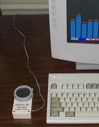Since October 16th, 1998, I've run an Aware Electronics RM-80 radiation monitor pretty much continuously, connected to a serial port on a 1992 vintage 486/50 machine. The RM-80 uses a 7313 pancake Geiger-Müller tube. The tube is halogen quenched and has a minimum dead time of 30 µS, with a mica window which allows alpha particles to pass. The computer interface generates high voltage for the tube from the Data Terminal Ready and Request to Send pins of the serial port and toggles the state of the Ring Indicator line whenever a count is detected. The serial port can be programmed to interrupt on changes in the state of this signal, making it straightforward to implement radiation monitoring in software. Tube sensitivity, calibrated with Cesium-137 (¹³⁷Cs), is 3.54 µR/hour per count per minute.

The second generation HotBits generator uses an RM-80 detector illuminated by a 5 microcurie ¹³⁷Cs check source. I decided to attach the HotBits spare detector to a PC and let it run as a background radiation monitor, as much as anything to let the detector run for a while to guard against “infant mortality” in any of its components, should it have to take over for the in-service detector. Aware Electronics supplies the detector with a DOS driver program called AW-SRAD, which I used to log the number of counts per minute, logging the collected data to files in CSV format.

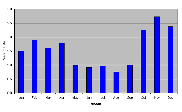
Database Coverage

Here's a plot that shows the extent of coverage by month over the period I monitored background radiation. The month of May, for example, has just about one year's complete data (this doesn't necessarily mean all of May for one year—it might be half of May in 1999 and half in 2000, for example). November has the greatest coverage, in excess of 2.5 years of data. The summer months have the least coverage due to vacations and other circumstances which caused me to shut down the machine connected to the detector. Since we're examining only diurnal variations—change in flux within a day—the uneven coverage over the months shouldn't be a problem. If we wanted to explore, for example, whether any diurnal variation we detected varied from month to month, it would be best to extract a subset of the data weighted equally by month, ideally with full coverage of each day of the solar year even though the days may be taken from different years.

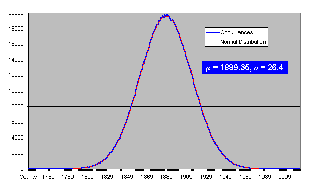
Counts per Minute Histogram

The first obvious step in reducing the data is to plot a histogram showing the distribution of counts per minute; the vertical axis is the number of minutes in the database in which the number of counts on the horizontal axis were recorded. The histogram table is reproduced in the bar at the right and plotted below.

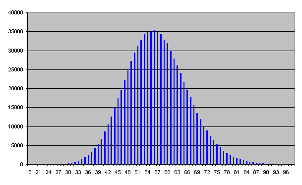
At first glance, this looks like the Gaussian “bell curve” you'd expect for a random process. At second glance, however, it doesn't…note that the “tail” on the right hand side, corresponding to larger numbers of counts per minutes appears distinctly longer and “fatter” than the tail on the left side. Still, let's proceed for the moment on the assumption that we do have a Gaussian distribution and calculate the mean and standard deviation from the data set. Crunching the numbers, we find a mean value of 56.65 counts per minute with a standard deviation of 9.31. We can then plot this Gaussian (normal) distribution as a red line superimposed on the histogram of experimental results.

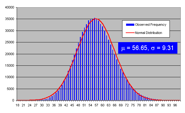
This makes it even more apparent that there's something happening which isn't “perfectly normal”. Note how the excess on the high end of the histogram pulls the best-fit normal distribution to the right of the actual data distribution, with the histogram bars to the left of the mean consistently exceeding the value of the normal curve and those to the right falling below.

You might be inclined to wonder just how closely we should expect experimental results like these to approximate a normal distribution. Could the observed deviation be nothing more than a statistical fluke? No…compare the fit of the background radiation histogram above with the the plot below of a data set of comparable size collected using the same detector but, instead of monitoring background radiation in counts per minute, measuring counts per second with the detector illuminated by the HotBits Cesium-137 source. Although this data set necessarily includes background radiation as well as counts due to the radiation source, with about 2000 counts per second from the ¹³⁷Cs source, the roughly one count per second from background radiation has a negligible influence on the results.

In the radiation source data set we see an essentially perfect fit of the expected normal distribution to the experimental data. This makes it quite clear that there's something curious going on with the background radiation data. But what?

The Two Population Hypothesis

One way we might end up with the kind of asymmetrical distribution we observe for the background radiation is if the radiation flux we're measuring is composed of two separate components, or populations, each individually normally distributed, but with different peak value, mean, and standard deviation. Suppose, for example, that the background radiation the detector measures is the sum of that due to decay of heavy elements (principally thorium and daughter nuclides) in the immediate vicinity (the earth beneath the detector and the structure of the building in which it is located) and a less intense cosmic ray flux which occurs in sporadic bursts with a greater mean value than the terrestrial flux. (At this point I'm simply suggesting these sources to illustrate how the background radiation might be composed of two (or more) separate populations with different statistics; I'm not identifying them as the actual components.)

Here's a “toy model” which illustrates how this might work.

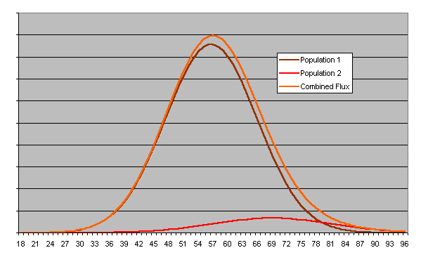
Let the brown curve labeled “Population 1” represent the terrestrial component of background radiation. It has a mean value of around 58 counts per minute and exhibits a precisely Gaussian distribution with total flux equal to the area under the brown Population 1 curve. We take the red “Population 2” curve to represent the supposed cosmic ray flux. This also has a normal distribution, but with a mean value of about 70 counts per minute, a greater standard deviation (resulting in a broader distribution curve), and a total flux only about one tenth that of Population 1.

Since counts resulting from the two populations cannot be distinguished by our simple detector, what we observe is the sum of the two populations, shown as the orange “Combined Flux” curve. Note the strong resemblance between this curve and the histogram plot from the detector; while Population 1 dominates the result, the contribution of Population 2 lifts and extends the high end of the combined distribution, precisely as we observed in the experimental data set.

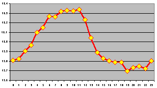
Radiation by Local Solar Time

Next I tried binning the results hourly by local solar time. The following chart shows the results, plotted in terms of average background radiation flux in micro-Roentgens per hour. (The average background radiation of 16.2 µR/hr—142 mR per year—may seem high, but my detector is located at an altitude of 800 metres above sea level. Both the soft and hard [primarily muon] components of cosmic rays are absorbed by the atmosphere, so at a higher altitude more they are more intense. At sea level, cosmic rays contribute about 30 mR/year, but at the 10 km altitude commercial jet aircraft fly, cosmic radiation accounts for about 2000 mR/year; more than 60 times as intense.) When I plotted the hourly local time averages, I obtained the following result.

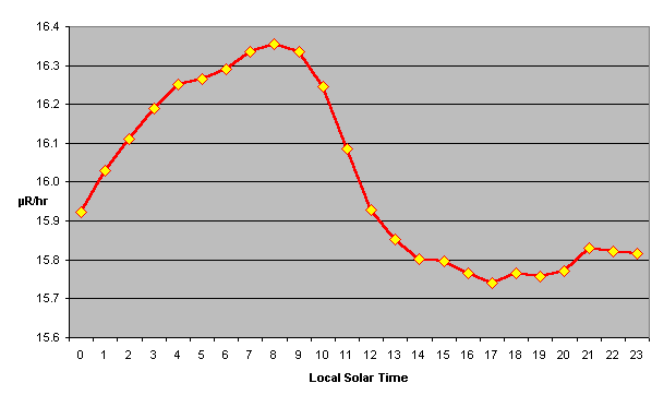
I've read about variations in cosmic ray flux varying with latitude, in Easterly and Westerly incidence, the solar cycle, and changes in the geomagnetic field, without a mention of a diurnal cycle, yet this plot appears to show a sinusoidal variation, with a magnitude variation between the highest three-hour period and the lowest of almost 6% of the mean value and, further, the trough in the curve seems to be about 12 hours from the peak.

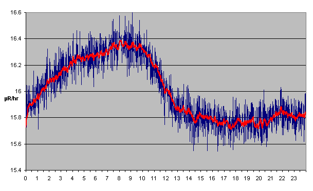
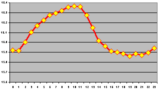
To explore whether this might be nothing but an artifact or statistical fluctuation, I then re-binned the same data minute by minute, resulting in the following plot, in which the blue curve is the raw minute-binned data and the red curve is the same data filtered by an exponentially smoothed moving average with a smoothing factor of 0.9.

Randomly selected data subset

Well, it still looks credibly sinusoidal, with the maximum and minimum at about the same point. As we all know, the human eye and brain are extraordinarily adept at seeing patterns in random data. So let's try another test frequently applied as a reality check when apparently significant results appear in a data set. The chart at the left was created by randomly selecting 25% of the points appearing in the complete data set and plotting them hour by hour. We find that the selection has little effect on the shape of the curve or the location of its maximum and minimum.

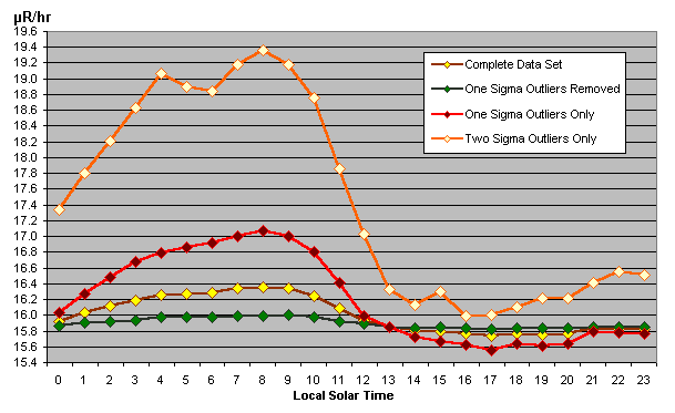
Outliers removed.

Next, I decided to explore whether the apparent sinusoidal variation might disappear if I discarded outlying values, which might conceivably vary differently in time than those which make up the bulk of the database. I pruned the bell curve at one standard deviation, then used the remaining data to prepare the plot at the left. As you can see, the case for a sinusoidal variation is eroded somewhat, but the general shape, magnitude, and location of extrema is conserved.

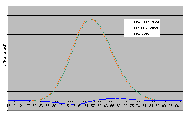
Outliers and Populations

The fact that removing the outlying values reduced the diurnal variation in the above plot suggests that we may indeed have two populations contributing to the observed flux, with the population responsible for the outlying values containing more diurnal variation than that near the mean. To investigate this further, I passed the data set through a variety of filters and prepared the following plot.

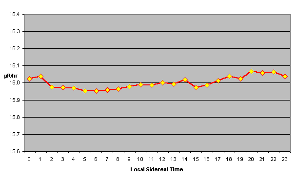
In the Stars?

Finally, I decided to plot the average radiation flux against local sidereal time. Sidereal time tracks the position of the distant stars as viewed from a given point on the Earth. At the same sidereal time, the same celestial objects (external to the solar system) will cross the celestial meridian above a given place on the Earth. Because the viewpoint of the Earth shifts as it orbits the Sun, the sidereal day (time between successive meridian crossings of a given star) is about 4 minutes shorter than the solar day (mean time between solar meridian crossings). Correlation with the sidereal period is powerful evidence for a distant source as the cause of a given effect. For example, it was correlation with the sidereal period which provided early radio astronomers evidence the centre of the galaxy and Crab Nebula were celestial sources of the noise they were monitoring. Here's a plot of average radiation flux by sidereal time.

What's Going On Here?

Darned if I know! The floor is open to inference and speculation.

First of all, I think it's reasonable to assume that any diurnal variation, should such exist, is due to cosmic rays. The balance of background radiation is primarily due to thorium, radon, and daughter nuclides in the local environment. Where I live, in the Jura mountains of Switzerland, subterranean rocks are almost entirely limestone, which has little or no direct radioactivity (as opposed to, for example, granite), nor radon precursors. In such an environment, it's hard to imagine a background radiation component other than cosmic rays which would vary on a daily basis. (This would not be the case, for example, in a house with a radon problem, where you would expect to see a decrease when doors and windows were opened during the day.)

If the effect is genuine, and the cause is cosmic ray flux, what are possible causes? The two which pop to mind are atmospheric density and the geomagnetic field. During the day, as the Sun heats the atmosphere, it expands. If you're at sea level, the total absorption cross section remains the same, but the altitude at which the primary cosmic ray first interacts with an atmospheric atom may increase. Further, an increase in atmospheric temperature may change the scale height of of the atmosphere, which would perturb values measured at various altitudes above sea level. We could explore temperature dependence by comparing average background radiation in summer and winter months.

Let's move on to the geomagnetic field. It's well documented that the Earth's magnetic field and its interaction with the Sun's create measurable changes in cosmic ray incidence, since the proton and heavy ion component of primary particles is charged and follows magnetic field lines. As any radio amateur or listener to AM radio in the 1950s knows, the ionosphere changes dramatically at night, allowing “skip propagation” of medium- and high-frequency signals far beyond the horizon. Perhaps this effect also modifies the geomagnetic field, affecting the number of charged cosmic rays incident at a given location.

If there is a diurnal effect, why on Earth should it peak around 07:00 local time? Beats me.

References

Clay, Roger, and Bruce Dawson. Cosmic Bullets. Reading, MA: Addison-Wesley, 1997. ISBN 978-0-7382-0139-9.

Wheeler, John Archibald, and Kenneth Ford. Geons, Black Holes, and Quantum Foam: A Life in Physics. New York: W.W. Norton, 1998. ISBN 978-0-393-31991-0.

Download Raw Data and Analysis Programs

If you'd like to perform your own investigations of this data set, you can download the data and programs used in preparing this page. The 2.8 Mb Zipped archive contains the raw data in rad5.csv and a variety of Perl programs which were used to process it in various ways. There is no documentation and these programs are utterly unsupported: you're entirely on your own.