![]()
Most computer applications specify colour in three-component systems such as RGB, HLS, or HSV. Derived from the mechanisms of human colour perception, these colour spaces map relatively straightforwardly onto display and printing technologies.
While human colour perception is well modeled by such systems, the physical interaction of light and matter is far more complicated. To correctly display the effects of dispersion in refractive media, diffraction, or absorption by nontrivial filters, image synthesis tools must consider the spectrum of the electromagnetic radiation and the spectral dependence of its absorption, reflection, and other interactions with objects; perceptual abstractions such as RGB are inadequate. A task as simple as rendering a scene under a variety of light sources: daylight, incandescent and fluorescent indoor lighting, and mercury and sodium vapour street lights cannot be accomplished without knowing the spectra of light sources and the spectral response of pigments.
Once the spectrum of the light impinging upon a point in the image plane is known, the eye's perception of that spectrum must be determined. Finally, display arguments must be calculated which evoke that perception in the viewer.
This article explains how, given light with an arbitrary spectrum, first to determine the CIE X, Y, and Z values which characterise a standard human observer's perception of its colour, then to calculate corresponding R, G, and B values for a display device with known primary colours. A companion C program illustrates the techniques and contains functions you can use to render spectra in your own programs.
We define a spectrum as a function P(λ) which gives, for any wavelength λ in the human visual range of 380 through 780 nanometres (nm), the power emitted per small constant-width wavelength interval centred about λ, normally in units of watts per nm.
Emission spectra of light sources and transmission, reflection, and absorption spectra of materials are usually determined empirically by spectrophotometry and specified as a table of measurements at wavelength intervals, frequently 5 nm, throughout the visual range.
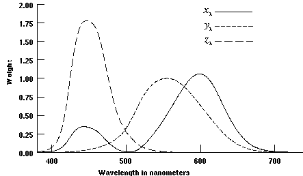
Figure 1.
CIE colour matching functions
x̅λ,
x̅λ,
z̅λ.
The CIE colour matching functions (Figure 1) x̅λ, x̅λ, and z̅λ give the relative contributions of light with wavelength λ to the CIE tristimulus values X, Y, and Z. The colour matching functions were determined by measuring the mean colour perception of a sample of human observers over the visual range from λviolet=380 to λred=780 nm. To calculate CIE X, Y, and Z values for light with spectrum P(λ) we sum, over the visual range, the products of the colour matching function weights at each wavelength and the intensity emitted at a constant narrow wavelength interval centred there:
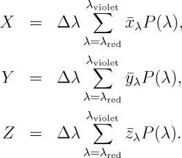 |
(1) |
|---|
For most applications sampling wavelength bands 5 or 10 nm
apart is adequate; (CIE 1971) and (CIE 1986) provide colour
matching tables with 1 nm resolution. The table
cie_colour_match in the
companion C program gives the CIE colour
matching functions every 5 nm.
The CIE Y value is a measure of the perceived luminosity of the light source—how bright it appears to an observer (to a first approximation; nonlinearities in the human visual system create a host of higher-order complexities). In rendering, we're usually interested only in relative luminosities so we can ignore absolute values of Y and simply scale luminosities between user-defined minimum and maximum brightnesses.
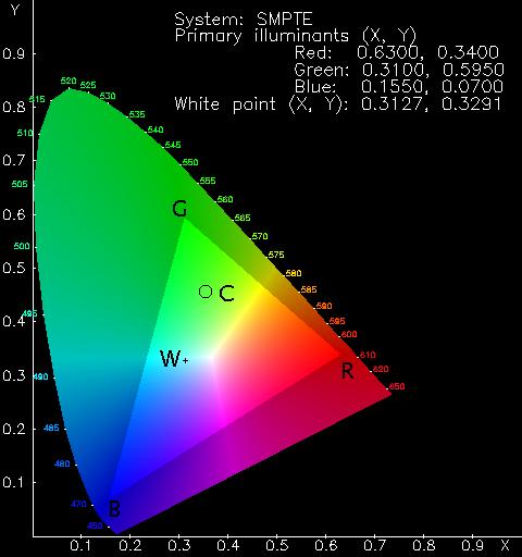
Figure 2. CIE chromaticity diagram. Pure spectral colours lie on the curved border of the “tongue”, labeled by wavelength. R, G, and B are the SMPTE primaries. W marks the SMPTE white point, CIE Illuminant D65. C is a colour which can be generated by mixing R, G, and B; it is said to lie within the colour gamut they define.
The X and Z components give the colour or chromaticity of the spectrum. Since the perceived colour depends (again, with the usual simplifications) only upon the relative magnitudes of X, Y, and Z, we define its chromaticity coordinates as:
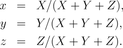 |
(2) |
|---|
Now since
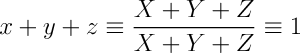
z may be obtained from x and y by:
![]()
and hence, chromaticity coordinates are usually given as just x and y.
If an output device accepts CIE colour specifications directly and transforms them into its colour gamut, we've nothing more to do. Usually, however, displays and printers require device-specific colour specifications in systems such as RGB or CMYK, requiring us to convert the CIE perceptual colour into device parameters.
| Red | Green | Blue | White Point | |||||
|---|---|---|---|---|---|---|---|---|
| System | xr | yr | xg | yg | xb | yb | xw | yw |
| NTSC | 0.67 | 0.33 | 0.21 | 0.71 | 0.14 | 0.08 | 0.3101 | 0.3162 |
| EBU (PAL/SECAM) | 0.64 | 0.33 | 0.29 | 0.60 | 0.15 | 0.06 | 0.3127 | 0.3291 |
| SMPTE | 0.630 | 0.340 | 0.310 | 0.595 | 0.155 | 0.070 | 0.3127 | 0.3291 |
The CIE Y component indicates the intensity of the light and the chromaticity coordinates x and y its colour in the CIE colour diagram (Figure 2). An RGB display mixes three primary colours, each of which is described by its CIE x and y (and implicitly z) coordinates. The three primaries define a triangle on the CIE diagram—any colour within it can be formed by mixing them. Table 1 lists the CIE x and y coordinates of the phosphors and reference white points of various broadcast systems. As noted in (Martindale and Paeth 1991), the NTSC primaries aren't remotely similar to those used in modern displays. Regrettably, the specifications of RGB monitors rarely include phosphor chromaticities, so unless you're prepared (and equipped) to calibrate the phosphors yourself, you're forced into choosing a “reasonable” set. Martindale and Paeth recommend calibrating to the SMPTE primaries, which are close to the EBU primaries used in PAL and SECAM broadcasting.
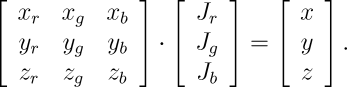
The amount of each primary to mix to yield a CIE colour with a given x, y, and z is the unknown J vector in the equation:
 |
(3) |
|---|
Solving for Jr, Jg, and Jb gives the weighting of Red, Green, and Blue primaries which yield the desired x, y, and z or, in other words, the coefficients of a linear combination of the primaries' chromaticity coordinates. The absolute intensity may then be adjusted based on the Y component (luminosity). The linear RGB values will require gamma correction if the display device has nonlinear response (non-unity gamma).
If any of Jr, Jg, or Jb are negative, the colour expressed by the x, y, and z chromaticity coordinates cannot be created by mixing the given primary colours; it lies outside the triangle they form in the CIE diagram.
The handling of colours unrepresentable on a given output device varies from application to application. If precise appearance must be maintained, asking the user to choose another colour may be appropriate. Less demanding applications may wish to replace the requested colour with a displayable approximation. A variety of schemes can be used to map unrepresentable colours into a device's gamut. An approach which often yields acceptable results is reducing the saturation of the requested colour until it falls within the RGB gamut. Recall that the curved outline of the CIE “tongue” diagram represents pure spectral—and therefore fully saturated—colours. A colour outside the RGB primary triangle will thus always be more saturated than can be displayed, and consequently must be approximated by a less saturated colour.
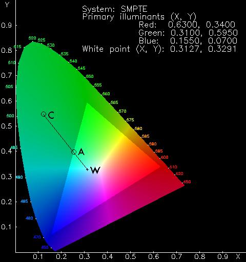
Figure 3. The requested chromaticity C cannot be achieved by mixing the given RGB primaries. Desaturating chromaticity C by mixing with the white point chromaticity W yields A, a within-gamut approximation of C.
Figure 3 demonstrates one way to accomplish this desaturation.
Requested colour C falls outside colour gamut RGB. The
line between the white point of the colour system W and
C includes, in the CIE diagram, all possible mixtures of
C and W. The point A where this line
intersects the RGB triangle is then the most saturated colour in
the direction of C representable within the gamut. The
function constrain_rgb in the
accompanying C program uses this technique
to approximate out-of-gamut colours.
Composite video encoding systems such as NTSC, PAL, and SECAM further restrict the colour gamut. Some bright, highly saturated colours accessible by mixtures of these systems' primaries are, nonetheless, “unencodable” due to limitations of bandwidth and modulation. In (Martindale and Paeth 1991) the authors describe the encoding limitations of various television systems and provide an algorithm which detects unencodable (“hot”) pixels and alters them into encodable replacements by reducing their luminance or saturation.
The spectral composition of many light sources is complicated and must be tabulated from photometric measurements. One useful family of light sources whose spectrum can be expressed as a simple function is the Planckian or black body radiators. The spectrum emitted by an ideal black body is determined entirely by its temperature; many natural and artificial light sources can be approximated by black body radiators of various temperatures.
| Source | Temperature, °K |
|---|---|
| Candle flame | 1900 |
| Sunlight at sunset | 2000 |
| Tungsten bulb—60 watt | 2800 |
| Tungsten bulb—200 watt | 2900 |
| Tungsten/halogen lamp | 3300 |
| Carbon arc lamp | 3780 |
| Sunlight plus skylight | 5500 |
| Xenon strobe light | 6000 |
| Overcast sky | 6500 |
| North sky light | 7500 |
For a ideal black body at temperature T (degrees kelvin), the emittance at a given wavelength λ (metres) is calculated by Planck's radiation law:
 |
(4) |
|---|
where Pλdλ is the hemispherical flux density in watts per square centimetre in the wavelength range between λ and λ+dλ. Constants c1 and c2 are:
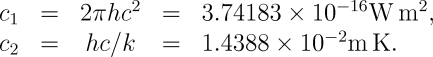
To determine the CIE XYZ coordinates of a black body with
temperature T, we use Eqs. (1) to sum, across the visual
spectrum, the products of the CIE colour matching functions and
the black body power spectrum from Eq. (4). In the
accompanying C program, this is performed
by spectrum_to_xyz which is passed the function
argument bb_spectrum which evaluates Planck's law
per Eq. (4). Since we're only interested in the colour of the
black body and not its absolute luminosity, we ignore the
Δλ terms in Eqs. (1) as they cancel when we compute
chromaticity coordinates with Eqs. (2).
Having found the chromaticity coordinates x, y,
and z, we must next convert them to RGB intensities in a
chosen colour system. The function xyz_to_rgb
solves Eq. (3) for Jr, Jg,
and Jb—the amount of each primary to
mix. If the colour lies inside the triangle formed by the
primaries, all the J weights will be nonnegative. If one
of the J values is negative, the colour falls outside the
RGB gamut (the negative J indicates we would have to
subtract that primary to obtain the requested x,
y, and z); the C function
inside_gamut performs this test.
If the requested colour is outside the gamut, the function
constrain_rgb replaces it with the nearest
within-gamut colour by mixing it with the colour system's white
point (see Table 1 and Figure 3). Finally, we print the CIE and
RGB colours of a black body with the given temperature,
indicating whether gamut limitations required desaturating the
RGB mixture. The chromaticity coordinates thus calculated are
in excellent agreement with the black body colourimetry
published in (Hunt 1987, page 196).
(CIE 1971). Commission Internationale de l'Éclairage (CIE). Publication No. 15, Colorimetry, 1986, 1971.
(CIE 1986). Commission Internationale de l'Éclairage (CIE). Standard on Colorimetric Observers, CIE S002, 1986.
(Hunt 1987). R.W.G. Hunt. Measuring Colour. Ellis Horwood Limited, 1987.
(Martindale and Paeth 1991). David Martindale and Alan W. Paeth. Television Color Encoding and “Hot” Broadcast Colors. In James Arvo, editor, Graphics Gems II, pages 147–158. Academic Press, Boston, 1991.
![]()
Last revised: March 9th, 2003
Documentation updated: July 8th, 2017