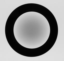
Schneider IIIb Centre Filter
Wide angle lenses, especially those used in medium- and large-format photography, frequently do not uniformly illuminate the entire film plane. Instead, they “vignette” the edges and corners of the image, substantially reducing the light reaching the film there.
|
Schneider IIIb Centre Filter |
The traditional solution for this is to attach a “centre filter” to the lens. This is a neutral density filter with maximum density at the optical axis of the lens, clear at the periphery, with density varying inversely to the vignetting of the lens. A centre filter has many advantages: not only does it automatically correct for full-frame images but, since it's fixed to the front of the lens, it also compensates for the off-centre vignetting which occurs when camera movements are employed for perspective or plane of focus adjustment.
But there are disadvantages as well. Many centre filters require a 1.5 or 2 f-stop filter factor adjustment, which may, in turn, necessitate a shutter speed so slow (since wide angle lenses, even with centre filters, are best used at apertures of f/16 or smaller) that hand-holding the camera is impossible and motion blur becomes a problem when photographing moving objects.
With the wide latitude of present-day film and the colour (or
grey-scale) depth of film scanners, it's possible to simulate
the effect of a centre filter after the fact by applying an
equivalent transform to a raw image taken without the filter.
pnmctrfilt applies a centre filter transform to a grey
scale or RGB image, allowing you to specify the density, power
of the density curve, image circle radius, and optionally
shift the centre of the filter to compensate for camera
movements.
A concrete example of the use of pnmctrfilt to process a real world image may help to clarify the abstract discussion above. Here's an image I shot in early October 2002 showing a coastline eroding into a beach below with a magnificent cloudscape above. I exposed this image on Kodak Ektachrome 100 transparency film in 6×9 cm format on 120 roll film with my ALPA 12 SWA and Rodenstock Apo-Grandagon f/4.5 35mm focal length super wide-angle lens at f/16 and 1/125 second. Now I have the appropriate centre filter for this lens, (Rodenstock 1094.2403.139), but it has an aperture correction factor of 1.5 f-stops, which means at a constant f-stop I'd need to increase the exposure time by a factor of three to compensate for the filter.
Let's be realistic. You need to stop down a lens like the Rodenstock
to around f/16 to get decent sharpness and coverage. If you tack on
1.5 stops of filter factor, there's no way you can
hand-hold an exposure like this and get the kind of sharpness
that the lens, camera, and film can deliver, and which this extraordinarily
complex image requires. (This landscape is dynamic—you can
see the sand filtering down from the eroding cliff and hear the
tick-tack of the eroded rocks falling onto the talus slope. Video might be
a better medium to capture it, but I chose the freeze-frame of a short
exposure to fix it in time. There was a stiff wind blowing from left
to right along the beach, making it even more difficult to hand-hold
the camera, and making the sand plumes swirl rapidly. I'd have
gotten less vignetting and a marginally sharper image at f/22, but
I decided that going to 1/60 second ran a larger risk to sharpness
than the larger aperture.)
Given the constraints, there's no way I could afford 1½ stops of centre filter factor. Even if I'd had the centre filter with me, tripling the exposure time would have wrecked the sharpness which is the theme of this image (in the original transparency, you can see individual grains of sand in the near field). Here's a scan of the Ektachrome transparency. The original scan was a 5312×3541 pixel TIFF file with 24 bits per pixel of colour depth, resulting in a 56 megabyte image file.
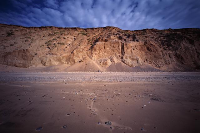
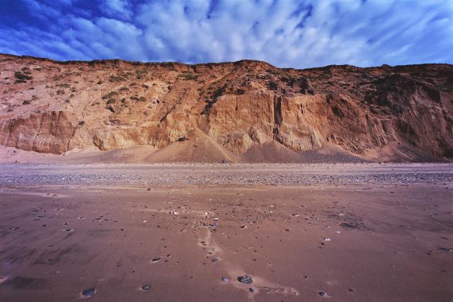
You can see the vignetting here. It's even more obvious in the transparency, but discussing that would get us into issues of display gamma, and we don't want to go there. Here's the result of processing this image with pnmctrfilt with a linear filter of density 5, greater than the attenuation of the centre filter recommended by Rodenstock for this lens. With the original image named scan03.tif, I used the following Netpbm pipeline to create the image below; I'll explain each step following the image resulting from this process.
    tifftopnm scan03.tif    |\	    # (1)
    pnmdepth 65535  	    |\	    # (2)
    pnmscale -width 640     |\	    # (3)
    pnmctrfilt --density 5  |\	    # (4)
    pnmdepth 255 >img03.ppm         # (5)
The img03.ppm file created by this pipeline was then brightness and contrast adjusted using The Gimp, based on interactive feedback, and saved as the JPEG file which appears below.
Steps in the processing this image were as follows:
1. tifftopnm converts the TIFF image scanned by the digital photo lab to a portable pixmap compatible with the Netpbm utilities.
2. Since the image was scanned with only 8 bits of resolution for each of the RGB colour channels, pnmdepth is used to widen the colour resolution to 16 bits per channel. This avoids round-off induced errors in the subsequent steps.
3. The image is re-scaled from the original high resolution scan to a 640 pixel width image suitable for inclusion in this Web page. If you envision subsequent image processing or wish to make a print of the image, you should leave it in the original scan resolution to avoid loss of detail.
4. Now we're ready to apply the centre filter. The centre filter Rodenstock recommend for this lens has a filter factor of 3, but like most centre filters, it doesn't entirely correct for vignetting. Here we use a virtual filter with a more accurate density of 5, which would would be hopeless as an optical filter. An excellent way to evaluate the effect of the centre filter parameters is to process the resulting image with a histogram equalising filter such as pnmhisteq which will emphasise any residual vignetting.
5. Many image processing programs can't cope with Netpbm files with more than 8 bits per colour channel so we reduce the colour resolution to 8 bits per pixel before exporting the image for further processing. The version of The Gimp I used to produce this image didn't understand 16 bit colour PPM files; if your image processing program does, there's no need to reduce the colour depth. If you wish to post-process the image with a program that doesn't read Netpbm files, you'll need to translate the file to a format it can read with an export filter such as pnmtotiff.
Processing an image with pnmctrfilt reduces the intensity of pixels at the centre of the filter by the specified density. This results in the image utilising less than the full intensity gamut. In many applications it makes sense to pass the centre filtered image through pnmnorm to stretch its intensity back into the full available range. For some images, however, pnmnorm produces results which are too contrasty; in such cases it's best to adjust the brightness and contrast with an interactive image processing program.
Remember that photography is an art as much as a science! Ansel Adams likened a negative to a musical score, with the print the performance. With today's digital image processing tools, we can easily create visual effects which would have been extraordinarily difficult or impossible in the darkroom. While there's nothing wrong (and much to be said) for precise calibration of vignetting, correction for nonlinearities in scanners and printing processes, etc., one shouldn't forget that the ultimate purpose of any photograph is to transmit a state of mind to the person who views it. If some residual vignetting acts to focus the viewer on the centre of the image and that's what you intend, then by all means leave it in!
If you evaluate the results of your image processing on a computer screen before sending it to a printer (or taking it to a service bureau to produce an exhibit print), be careful not to be deceived by subtle properties of computer screens. First of all, there's gamma, but I promised not to talk about that. Nonetheless, you should be aware that the inherent contrast of various computer displays differ and, in turn, may be very different from those of print processes. “Colour matching” technologies attempt to avoid these problems but, at this writing, they're in their infancy. Be prepared for some stinker prints until you learn to compensate. If you're using a service bureau for your prints, it's wise to order some cheap small prints to get the settings right before springing for gallery prints which will bust your budget if they end badly.
One particular hazard in correcting images for vignetting applies to users of LCD flat-panel display screens on laptop and trendy desktop computers. These displays have their own vignetting—if you're looking at the centre of the screen, pixels toward the corners will appear darker. If you move your head so you're looking directly at the corner of the screen, pixels there will appear bright while the rest of the screen will look subdued. Be careful not to confuse apparent vignetting due to your display with actual vignetting of the processed image. Testing with histogram equalised images (pnmhisteq) can help with this.
A variety of command line options permit you to adjust various aspects of the filter applied by pnmctrfilt. For a detailed description, see the OPTIONS section in the manual page below. This section describes the options in a narrative form and gives examples of typical option specifications.
The -density option controls the degree of intensity attenuation by the filter at its point of maximum density. The default density is 2, which corresponds to an optical filter with a 1 f-stop filter factor. Increase the density to compensate for a greater degree of vignetting; reduce it for less. Setting the density less than 1 results in an inverse centre filter which will increase vignetting in the image.
The -power option determines the rate at which the filter intensity falls off from the point of maximum density toward the edges, expressed as a power factor. The default of 1 yields a linear reduction in filter density with distance from the centre. Power factors greater than 1 cause a faster fall-off (for example, a power of 2 causes the density to decrease as the square of the distance from the centre) and causes the effect of the filter to be concentrated near the centre. Powers less than 1 spread out the density of the filter toward the edges; a power of 0.5 causes the density to fall as the square root of the distance from the centre.
The -radius option specifies the radius, as a multiple of the half diagonal measure of the image, at which the density of the filter falls to zero (or, in other words, becomes transparent). The default value of 1 specifies a filter which, if centred upon the image, is transparent at its corners. A radius specification greater than 1 extends the effect of the centre filter beyond the edges of the image, while a radius less than one limits the filter's action to a region smaller than the image. When compensating for vignetting by lenses used with large format and some medium format cameras, the default radius factor of 1 is rarely correct! These lenses often “cover” an image circle substantially larger than the film to permit camera movements to control perspective and focus, and consequently have a vignetting pattern which extends well beyond the edges of the film, requiring a -radius setting greater than 1 to simulate a centre filter covering the entire image circle.
The only way to be sure which settings of -density, -power, and -radius best compensate for the actual optical characteristics of a given lens is to expose a uniformly illuminated scene (for example, a grey card lit by diffuse light) and perform densitometry on the resulting image. Failing that, or specifications by the lens manufacturer giving the precise degree of vignetting at one or more working apertures, you may have to experiment with different settings to find those which work best for each of your lenses. Fortunately, the response of the human eye is logarithmic, not linear like most digital imaging sensors, so you needn't precisely compensate for the actual vignetting to create images which viewers will perceive as uniformly illuminated.
If you're using a view camera with camera movements (shift and tilt of the lens plane with respect to the film plane), the optical axis of the lens (the line which passes through its centre) may not coincide with the centre of the film. If this is the case, vignetting by the lens will be shifted from the centre of the resulting image. You can compensate for this by specifying the position of the optical axis (centre of the vignetting pattern) in the image with the -xshift and/or -yshift options. Positive shifts move the centre of the lens to the right and down, while negative shifts move it to the left and up; the shift is specified in pixels. For example, suppose you've exposed a 56×84 mm image of a building, having shifted the lens upward 18 mm to show the full height of the building without causing vertical lines to converge, then scanned the image at a resolution of 100 pixels per millimetre, yielding a 5600×8400 pixel image. To align the centre filter with the optical axis of the lens, you'd then want to shift it upward 18 mm from the centre of the scanned image, or 1800 pixels at the resolution of the scan, which can be accomplished by specifying the -yshift -1800 option.
The following images illustrate the effect of various pnmctrfilt option settings. Each was created by generating a 256×256 pixel white image, then processing it with pnmctrfilt using the indicated options:
    ppmmake rgb:FF/FF/FF | \
        pnmctrfilt options | \
        pnmtopng >ofile.png
The options used to filter each image are given beneath it, with default values in grey type.

-density 2 -power 1 -radius 1 -xshift 0 -yshift 0 |

-density 2 -power 3 -radius 1 -xshift 0 -yshift 0 |
|

-density 2 -power 0.3 -radius 1 -xshift 0 -yshift 0 |

-density 5 -power 3 -radius 1 -xshift 0 -yshift 0 |
|

-density 2 -power 1 -radius 0.5 -xshift 0 -yshift 0 |

-density 2 -power 3 -radius 1 -xshift 64 -yshift 0 |
|

-density 2 -power 3 -radius 1 -xshift 0 -yshift -48 |

-density 0.5 -power 1 -radius 2 -xshift 0 -yshift 0 |
pnmctrfilt is an addition to the Netpbm image processing toolkit. In order to install and use it, you first need to obtain the current Netpbm source code and build executables for your computer. The Netpbm project is hosted on SourceForge, and the current source code archive may be downloaded from the following project page link.
Netpbm Project Page on SourceForge
The current release of Netpbm as of the writing of this document was version 10.12. Netpbm is mature, production software and changes only slowly, so you should have little if any difficulty integrating pnmctrfilt in subsequent versions.
Once you've downloaded the Netpbm source distribution, build executables for your system. Detailed instructions are provided in the doc/INSTALL and README files in the distribution directory tree. Users of many Linux distributions will be able to build with just the following two commands:
    ./configure
    make
If you're using a different flavour of Unix, you may need to install various software tools and libraries in order to build a full-featured version of Netpbm; see the doc/INSTALL and README files for details.
Once you've built Netpbm, download the source code for pnmctrfilt.c from the following link.
Source code for editor/pnmctrfilt.c: pnmctrfilt.tar.gz
This is a gzip-compressed tar archive which should be extracted in the root directory of the Netpbm distribution (the one containing the README file). It will install the source code file pnmctrfilt.c in the editor subdirectory where the other image transformation tools are kept.
Next, add pnmctrfilt to editor/Makefile as the last target listed under MATHBINARIES; this will cause the Makefile in the editor subdirectory to build the pnmctrfilt program. For version 10.12 of Netpbm the patch to editor/Makefile is:
   diff -r Onetpbm-12.12/editor/Makefile netpbm-10.12/editor/Makefile
   28c28
   <               pnmshear pnmstitch ppmlabel ppmntsc
   ---
   >               pnmshear pnmstitch ppmlabel ppmntsc pnmctrfilt
but you should edit the editor/Makefile yourself and make the equivalent change since it may have changed since this document was written.
Finally, in the root directory of the Netpbm distribution, re-build the package with:
make
which will build the newly-added pnmctrfilt utility. If all goes well, you may now proceed with installing the new version of Netpbm on your system. If you've a current version of Netpbm already installed (included, for example, with a Linux distribution), you may choose simply to copy the editor/pnmctrfilt binary to a directory on your PATH and continue to use the existing Netpbm binaries for the other programs.
Documentation for pnmctrfilt follows, in Netpbm manual page style.
Applies a centre filter transformation to PNM (usually PGM or PPM) images.
Wide angle lenses, especially those used in medium- and large-format photography, frequently do not uniformly illuminate the entire film plane. Instead, they “vignette” the edges and corners of the image, substantially reducing the light reaching the film there.
The traditional solution for this is to attach a “centre filter” to the lens. This is a neutral density filter with maximum density at the optical axis of the lens, clear at the periphery, with density varying inversely to the vignetting of the lens. A centre filter has many advantages: not only does it automatically correct for full-frame images but, since it's fixed to the front of the lens, it also compensates for off-centre vignetting when camera movements are employed for perspective or plane of focus adjustment.
But there are disadvantages too. Many centre filters require a 1.5 or 2 f-stop filter factor adjustment, which may, in turn, necessitate a shutter speed so slow (since wide angle lenses, even with centre filters, are best used at very small apertures) that hand-holding the camera is impossible and motion blur becomes a problem when photographing moving objects.
With the wide latitude of present-day film and the colour (or grey-scale) depth of film scanners, it's possible to simulate the effect of a centre filter after the fact by applying an equivalent transform to the raw image shot without the filter. pnmctrfilt applies a centre filter transform to a grey scale or RGB image, allowing you to specify the density, power of the density curve, and optionally offset the centre of the filter to compensate for camera movements.
Processing an image with pnmctrfilt reduces the intensity of pixels at the centre of the filter by the specified density. This will usually result in an image utilising less than the full gamut of intensity. In many applications it makes sense to pass the resulting image through pnmnorm to stretch its intensity back into the full range available.
The only parameter is the optional pnmfile to be read; if omitted or pnmfile is “-”, pnmctrfilt reads from standard input.
Copyright © 2003 by John Walker. The source code for this program is in the public domain. Executable versions of the program are subject to the licenses of all the libraries they incorporate.
| by John Walker January 7th, 2003 |
|