|
|
Nuclear Bomb Effects ComputerProduction Notesby John Walker |
|
|
|
Nuclear Bomb Effects ComputerProduction Notesby John Walker |
|
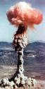
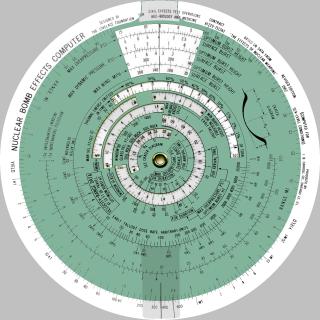
This online edition of the nuclear bomb effects computer was produced by scanning a 1962 second edition bomb computer slide rule from the Fourmilab Museum. The resulting images were processed with a variety of tools to create “component” images, which are assembled into the results generated for online requests with custom software. This document provides an overview of the image database production and request servicing processes.
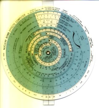
The plastic slide rule was scanned, front and back, with a Hewlett-Packard ScanJet
6300C colour scanner set at 600 dots per inch resolution. This produced images with
about 3150 pixels of resolution across the approximately 5 1/8 inch / 13 cm
base disc of the slide rule. A canonical radius of 1575 pixels was used for subsequent
processing of these scans. Some contamination of the inside of the scanner platen
apparently due to outgassing of plastic components contributed to the greenish
cast of the left side of the scanned images; this discolouration does not appear
on the actual slide rule. Because the colours were to be re-generated during the
subsequent image processing steps, this effect was ignored.
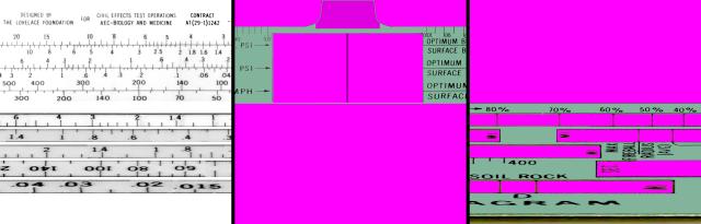
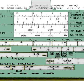
Each of the original scanned images was then “rectified”, transforming it from polar to
rectangular co-ordinates by logically “unwrapping it” around its centre, as defined by
the rivet about which the slide rule pivots. This was performed by a purpose-built utility,
ppmcirctorect,
added to the
Netpbm image
processing toolkit. The effect of this program can be thought of as
running a cursor with a line equal to the radius of the image around
a full circle in increments of one pixel measured at the
circumference, and for each step reading off the pixel from the disc
image beneath each radial dot on the cursor. This yielded images of
9896×1575 (the width being just 2 Pi times the radius) from each
scan; the image at the right is an excerpt of the rectified image
produced from the scan above. Note the expansion and distortion of
material as one approaches the centre (bottom of the rectified
image); the bar at the bottom is the extremely stretched out rivet.
This clip was taken around the overpressure window; note how this
window, which appears wedge-shaped in the scan, is rectangular when
transformed to this projection. The distortion, however bad it may
look, is completely reversible—pixels near the centre are
replicated, but nothing is lost when going back from a rectified
image to a polar projection. Transforming to the rectangular
projection drastically simplifies the subsequent image editing and
processing tasks, since image processing software understands
straight lines and rectangular boxes far better than polar
co-ordinates.
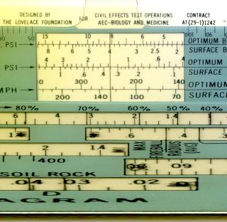
The functional components—each separate moving part of the slide rule—were then extracted, yielding rectified images of each component. Above, clips of the component images for the base plate, outer wheel, and inner wheel are shown, each corresponding to the extract from the composite rectified image in the previous section. Transparent windows in the overlay components are filled with magenta (HTML colour code #FF00FF), and portions which are transparent but which darken the material beneath (such as the cursor tab above the window in the outer wheel in the middle image), are darker shades of magenta with precisely equal red and blue colour components.
Since the windows in the rotating components do not expose the entire underlying scale on the base disc at any single rotation setting, the complete base plate image was assembled by compositing scale segments extracted from a total of twelve scans made with different rotations of the inner and outer wheels. This compositing was done with Jasc Paint Shop Pro (version 7), using its multiple layer and transparency features to guarantee precise alignment when adjacent segments of a scale were spliced together. Some of the windows in the rotating wheels have cursor lines which obscure underlying material on the base; these were removed by manual retouching, usually from an adjacent scan in which the same portion of the scale appeared unobstructed.
The wheel components, whose blue-green tint was captured unevenly by the scanner, were restored to a uniform shade by extracting the green channel from the colour image of the scan and processing it through another custom Netpbm program, ppmmidtone, which identified the range of grey scale values corresponding to the background of the wheel components, replacing pixels within that range with the desired colour.
A similar process was used to produce components for the base, curve, and cursor of the back of the slide rule. This was simplified by the lack of obscuration, complex window structure, and pastel tones on that side.
The parameters defining a problem to be solved are specified numerically, for example, yield in kilotons and range in miles. Rather than make the user play silly pixel-picking games to rotate the slide rule wheels to the correct values, we want to allow values to be entered directly and the wheels set accordingly. (This is something makers of pixel-oriented graphics software never seem to get—precisely specifying a position all too often amounts to a frustrating test of hand/eye co-ordination and the ability to click a mouse button without shifting its position. When whey will they learn that the trivial addition of allowing the user to enter pixel positions from the keyboard into the fields where they already display the position can reduce the difficulty and improve the productivity of this task by a factor of ten or more?)
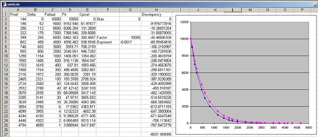
To permit specifying parameters numerically, we need to determine a function which maps parameters within the range covered by the scales on the slide rule into their pixel column (horizontal) co-ordinates within the appropriate component image. For each parameter, this function was determined empirically by entering parameter values and pixel numbers into an Excel spreadsheet, plotting the relationship in a chart, and then finding a function which reproduces at relationship to a high degree of precision. As it happens, all of the scales on the bomb computer which we wish to set are logarithmic, as a glance at the chart above reveals, so we need only determine the correct initial value and exponent. This was done by using the inverse of the function to map parameter values back to pixel co-ordinates, creating a table of the discrepancy between each measured and computed pixel location, summing the discrepancies, and then using the Excel “Goal Seek” mechanism to minimise the total discrepancy by adjusting the exponent. In the illustration above, I have deliberately entered an incorrect exponent so you can see the difference between the curves showing the measured (blue) and computed (purple) curves. Once the exponent has been optimised, the curves precisely overlap within the resolution of the plot. The result for this example, once the exponent is optimised, is that we can map a fallout dose rate in the arbitrary 1 to 10000 units used on the bomb computer scale into the pixel location on the scale with the expression (written as in the C programming language):
These mappings are not precise to the pixel; small discrepancies do exist. The bomb computer is a physical device, subject to the imprecision of the manufacturing process used to make it (mine is noticeably out of round, for example), and even the master image, which appears to have been laid out by hand, is not mathematically perfect. Any errors induced by slight discrepancies in the parameter to pixel function are entirely negligible compared to parallax errors setting and reading the physical slide rule and, in any case, pale into insignificance given the rough and tumble nature of estimations of weapons effects.
Using the empirically determined mapping functions to obtain the pixel columns for the user's problem inputs, we can then re-combine the rectangular projection components of the slide rule, shifted so the the settings for each line up at the same position. This is equivalent to rotating the wheels of the circular slide rule. The shifting is like a “circular shift” of a computer register—the rectangular image should be thought of as a cylinder with the pixels at the right and left edges adjacent to one another. When the image is shifted to the right, for example, pixels shifted out on the right appear at the left.
The shifting and composition of components is done with yet another custom
Netpbm program, ppmsliderule, which is called with a list of
component images and shift values. Components are logically
stacked, bottom to top, in the order specified on the command line, with
transparent and partially transparent areas (indicated by shades of
magenta) in components allowing the contents of lower layers to show
through. The image at the right a clip of the result of combining the
three front components of the slide rule, aligned as they were in the
scanned images shown at the top.
All that remains is to transform the merged rectangular image of the
correctly set slide rule back into a polar projection—to wrap it
back into the circular form whence it originated. This is done by
the same ppmcirctorect program used to make the rectangular
projections in the first place, invoked this time with an option
specifying the inverse transformation. The result of running this
program is shown at right, with the same settings and orientation as
the scanned image at the top to facilitate comparison. The details
of assembling and transforming the image for individual user requests
are attended to by bombcalc.pl, a Perl program invoked by
the CGI script that processes each request.
If you're interested in how the programs mentioned above work, or have a potential application of your own for them, you're free to download their source code from the following links. These programs are absolutely, utterly undocumented and unsupported—you are entirely on your own! Requests for information about or assistance regarding these programs will be silently ignored apart, perhaps, from quiet cackling.
Download:
|
|