Orbits in Strongly Curved Spacetime
Introduction
The display above shows, from three different physical perspectives,
the orbit of a low-mass test particle, the small red circle,
around a non-rotating black hole (represented by a grey
circle in the panel at the right, where the radius of the circle is
the black hole's gravitational radius, or
event horizon. Kepler's laws of planetary motion, grounded in
Newton's theory of gravity, state that the orbit of a test particle
around a massive object is an ellipse with one focus at the centre
of the massive object. But when gravitational fields are strong, as
is the case for collapsed objects like neutron stars and black
holes, Newton's theory is inaccurate; calculations must be done using
Einstein's theory of General Relativity.
In Newtonian gravitation, an orbit is always an ellipse. As the
gravitating body becomes more massive and the test particle orbits it
more closely, the speed of the particle in its orbit increases without
bound, always balancing the gravitational force. For a black
hole, Newton's theory predicts orbital velocities greater than the
speed of light, but according to Einstein's Special Theory of
Relativity, no material object can achieve or exceed the speed of light.
In strong gravitational fields, General Relativity predicts
orbits drastically different from the ellipses of Kepler's laws.
This page allows you to explore them.
The Orbit Plot
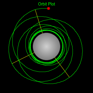 The panel at the right shows the test mass orbiting the black hole,
viewed perpendicular to the plane of its orbit. The path of the orbit is
traced by the green line. After a large number of orbits the display
will get cluttered; just click the mouse
anywhere in the right panel to erase the path and start over. When
the test mass reaches its greatest distance from the black hole, a
yellow line is plotted from the centre of the black hole to that
point, the apastron of the orbit. In Newtonian gravity,
the apastron remains fixed in space. The effects of General Relativity
cause it to precess. You can see the degree of precession in
the displacement of successive yellow lines (precession can be more
than 360°; the yellow line only shows precession modulo one
revolution).
The panel at the right shows the test mass orbiting the black hole,
viewed perpendicular to the plane of its orbit. The path of the orbit is
traced by the green line. After a large number of orbits the display
will get cluttered; just click the mouse
anywhere in the right panel to erase the path and start over. When
the test mass reaches its greatest distance from the black hole, a
yellow line is plotted from the centre of the black hole to that
point, the apastron of the orbit. In Newtonian gravity,
the apastron remains fixed in space. The effects of General Relativity
cause it to precess. You can see the degree of precession in
the displacement of successive yellow lines (precession can be more
than 360°; the yellow line only shows precession modulo one
revolution).
The Gravitational Effective-Potential
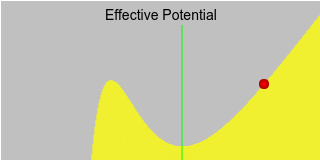 The panels at the left display the orbit in two more abstract ways.
The Effective Potential plot at the top shows the position
of the test mass on the gravitational energy curve as it orbits
in and out. The summit on the left side of the curve is unique to
General Relativity—in Newtonian gravitation the curve rises without
bound as the radius decreases, approaching infinity at zero. In Einstein's
theory, the inability of the particle to orbit at or above the
speed of light creates a “pit in the potential” near the black hole.
As the test mass approaches this summit, falling in from larger radii
with greater and greater velocity, it will linger near the energy
peak for an increasingly long time, while its continued angular motion
will result in more and more precession. If the particle
passes the energy peak and continues to lesser radii, toward
the left, its fate is sealed—it will fall into the black hole
and be captured.
The panels at the left display the orbit in two more abstract ways.
The Effective Potential plot at the top shows the position
of the test mass on the gravitational energy curve as it orbits
in and out. The summit on the left side of the curve is unique to
General Relativity—in Newtonian gravitation the curve rises without
bound as the radius decreases, approaching infinity at zero. In Einstein's
theory, the inability of the particle to orbit at or above the
speed of light creates a “pit in the potential” near the black hole.
As the test mass approaches this summit, falling in from larger radii
with greater and greater velocity, it will linger near the energy
peak for an increasingly long time, while its continued angular motion
will result in more and more precession. If the particle
passes the energy peak and continues to lesser radii, toward
the left, its fate is sealed—it will fall into the black hole
and be captured.
The Gravity Well
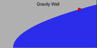 Spacetime around an isolated spherical non-rotating uncharged
gravitating body is described by Schwarzschild Geometry, in
which spacetime can be thought of as being bent by the presence of
mass. This creates a gravity well which extends to the
surface of the body or, in the case of a black hole, to oblivion. The
gravity well has the shape of a four-dimensional paraboloid of
revolution, symmetrical about the central mass. Since few Web
browsers are presently equipped with four-dimensional display
capability, I've presented a two-dimensional slice through the gravity
well in the panel at the bottom left. Like the energy plot above, the
left side of the panel represents the centre of the black hole and the
radius increases to the right. Notice that the test mass radius moves
in lockstep on the two charts, as the radius varies on the orbit plot
to their right.
Spacetime around an isolated spherical non-rotating uncharged
gravitating body is described by Schwarzschild Geometry, in
which spacetime can be thought of as being bent by the presence of
mass. This creates a gravity well which extends to the
surface of the body or, in the case of a black hole, to oblivion. The
gravity well has the shape of a four-dimensional paraboloid of
revolution, symmetrical about the central mass. Since few Web
browsers are presently equipped with four-dimensional display
capability, I've presented a two-dimensional slice through the gravity
well in the panel at the bottom left. Like the energy plot above, the
left side of the panel represents the centre of the black hole and the
radius increases to the right. Notice that the test mass radius moves
in lockstep on the two charts, as the radius varies on the orbit plot
to their right.
The gravity well of a Schwarzschild black hole has a throat
at a radius determined solely by its mass—that is the location of the
hole's event horizon; any matter or energy which crosses the
horizon is captured. The throat is the leftmost point on the gravity
well curve, where the slope of the paraboloidal geometry becomes
infinite (vertical). With sufficient angular momentum, a particle can
approach the event horizon as closely as it wishes (assuming it is
small enough so it isn't torn apart by tidal forces), but it can never
cross the event horizon and return.
Hands On
By clicking in the various windows and changing values in the controls
at the bottom of the window you can explore different scenarios.
To pause the simulation, press the Pause button at the
right; pressing it again resumes the simulation. Click anywhere in
the orbit plot at the right to clear the orbital trail and
apastron markers when the screen becomes too cluttered. You can re-launch
the test particle at any given radius from the black hole (with
the same angular momentum) by clicking at the desired radius in either
the Effective Potential or Gravity Well windows. The green line
in the Effective Potential plot indicates the energy minimum at which a stable
circular orbit exists for a particle of the given angular momentum.
The angular momentum is specified by the box at left in terms of the
angular momentum per unit mass of the black hole, all in
geometric units—all of this is explained in
detail below. What's important to note is that for orbits like those
of planets in the Solar System, this number is huge; only in strong
gravitational fields does it approach small values. If the angular
momentum is smaller than a critical value
( , about 3.464 for
a black hole of mass 1, measured in the same units), no stable orbits
exist; the particle lacks the angular momentum to avoid being
swallowed. When you enter a value smaller than this, notice how the trough in
the energy curve and the green line marking the stable circular orbit
disappear. Regardless of the radius, any particle you launch is doomed
to fall into the hole.
, about 3.464 for
a black hole of mass 1, measured in the same units), no stable orbits
exist; the particle lacks the angular momentum to avoid being
swallowed. When you enter a value smaller than this, notice how the trough in
the energy curve and the green line marking the stable circular orbit
disappear. Regardless of the radius, any particle you launch is doomed
to fall into the hole.
The Mass box allows you to change the mass of the black hole,
increasing the radius of its event horizon. Since the shape of the
orbit is determined by the ratio of the angular momentum to
the mass, it's just as easy to leave the mass as 1 and
change the angular momentum. You can change the scale of all
the panels by entering a new value for the maximum radius; this
value becomes the rightmost point in the effective potential
and gravity well plots and the distance from the centre of
the black hole to the edge of the orbit plot. When you change
the angular momentum or mass, the radius scale is automatically
adjusted so the stable circular orbit (if any) is on screen.
Kepler, Newton, and Beyond
In the early 17th century, after years of tedious calculation
and false starts, Johannes Kepler published his three laws of
planetary motion:
-
First law (1605): A planet's orbit about the Sun is an
ellipse, with the Sun at one focus.
-
Second law (1604): A line from the Sun to a planet sweeps out
equal areas in equal times.
-
Third law (1618): The square of the orbital period of a planet is
proportional to the cube of the major axis of the orbit.
Kepler's discoveries about the behaviour of planets in their
orbits played an essential rôle in Isaac Newton's formulation
of the law of universal gravitation in 1687. Newton's
theory showed the celestial bodies were governed by the same
laws as objects on Earth. The philosophical implications of
this played as key a part in the Enlightenment as did the
theory itself in the subsequent development of physics
and astronomy.
While Kepler's laws applied only to the Sun and planets, Newton's
universal theory allowed one to calculate the gravitational force and
motion of any bodies whatsoever. To be sure, when many
bodies were involved and great accuracy was required, the calculations
were
horrifically
complicated and tedious—so much so that
those reared in the computer age may find it difficult to
imagine embarking upon them armed with nothing but a table of
logarithms, pencil and paper, and the human mind. But performed they
were, with ever greater precision as astronomers made increasingly
accurate observations. And those observations agreed perfectly with
the predictions of Newton's theory.
Well,… almost perfectly. After painstaking observations
of the planets and extensive calculation, astronomer Simon Newcomb
concluded in 1898 that the orbit of Mercury was precessing 43
arc-seconds per century more than could be explained by the influence
of the other planets. This is a tiny discrepancy, but further
observations and calculations confirmed Newcomb's—the discrepancy was
real. Some suggested a still undiscovered planet closer to the Sun
than Mercury (and went so far as to name it, sight unseen,
“Vulcan”),
but no such planet was ever found, nor any other plausible explanation
advanced. For nearly twenty years Mercury's precession or “perihelion
advance” remained one of those nagging anomalies in the body of
scientific data that's trying to tell us something, if only we knew
what.
In 1915, Albert Einstein's General Theory of Relativity extended
Newtonian gravitation theory, revealing previously unanticipated subtleties of
nature. And Einstein's theory explained the perihelion advance of
Mercury. That tiny discrepancy in the orbit of Mercury was
actually the first evidence for what lay beyond Newtonian
gravitation, the first step down a road that would lead to
understanding black holes, gravitational radiation, and the source of
inertia, which remains a fertile ground for theoretical and
experimental physics a century thereafter.
Geometric Units
The force of gravity is so weak compared to the electromagnetic
force which binds objects on the human scale, and the speed of
light so great compared to velocities with which we're familiar, that
calculating the effects of general relativity, which involve
both the gravitational force and the speed of light, using
conventional units like grams, centimetres, and seconds usually
results in enormous or minuscule quantities cumbersome to
manipulate and difficult to understand intuitively.
If we're interested in the domain where general relativistic
effects are substantial, we're better off calculating with units
scaled to the problem. A particularly
convenient and elegant choice is the system of geometric
units, obtained by setting Newton's gravitational
constant G, the speed of light c,
and Boltzmann's constant k all equal to 1. We
can then express any of the following units as a length
in centimetres by multiplying by the following conversion
factors.
| Quantity |
Unit |
cm Equivalent |
| Time |
second |
2.997930×1010 cm/sec |
| Mass |
gram |
0.7425×10⁻²⁸ cm/g |
| Energy |
erg |
0.826×10−49 cm/erg |
| Electric charge |
e |
1.381×10⁻²⁸ cm/e |
| Temperature |
° Kelvin |
1.140×10−65 cm/°K |
The enormous exponents make it evident that
these units are far removed from our everyday experience.
It would be absurd to tell somebody, “I'll call you back
in 1.08×10¹⁴ centimetres”, but it is a perfectly
valid way of saying “one hour”. The discussion that follows
uses geometric units throughout, allowing us to treat mass,
time, length, and energy without conversion factors. To
express a value calculated in geometric units back to
conventional units, just divide by the value in the table
above.
The Gravitational Effective-Potential
The gravitational effective-potential for a test particle orbiting
in a Schwarzschild geometry is:
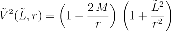
where  is
the angular momentum per unit rest mass expressed in geometric units,
M is the mass of the gravitating body, and r is the
radius of the test particle from the centre of the body.
is
the angular momentum per unit rest mass expressed in geometric units,
M is the mass of the gravitating body, and r is the
radius of the test particle from the centre of the body.
The radius of a particle from the centre of attraction evolves in
proper time τ
(time measured by a clock moving along with the particle)
according to:
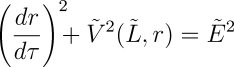
where  is the potential energy of the test mass at infinity per rest mass.
Angular motion about the centre of attraction is then:

while time, as measured by a distant observer advances according to:
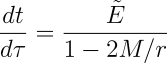
and can be seen to slow down as the event horizon at the gravitational
radius is approached. At the gravitational radius of 2M time,
as measured from far away, stops entirely so the particle never seems
to reach the event horizon. Proper time on the particle continues to
advance unabated; an observer on-board sails through the event
horizon without a bump and continues toward the doom which awaits
at the central singularity.
Circular Orbits
Circular orbits are possible at maxima and minima of the effective-potential.
Orbits at minima are stable, since a small displacement increases the
energy and thus creates a restoring force in the opposite direction.
Orbits at maxima are unstable; the slightest displacement causes the
particle to either be sucked into the black hole or enter a highly
elliptical orbit around it.
To find the radius of possible circular orbits, differentiate
the gravitational effective-potential with respect to the
radius r:
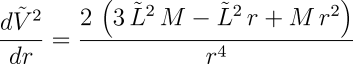
The minima and maxima of a function are at the zero crossings of its
derivative, so a little algebra gives the radii of possible circular
orbits as:
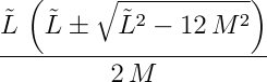
The larger of these solutions is the stable circular orbit, while the
smaller is the unstable orbit at the maximum. For a black hole, this
radius will be outside the gravitational radius at 2M, while
for any other object the radius will be less than the diameter of
the body, indicating no such orbit exists. If the angular
momentum L² is less than 12M², no stable orbit
exists; the object will impact the surface or, in the case of a
black hole, fall past the event horizon and be swallowed.
References
Click on titles to order books on-line from

|
- Gallmeier, Jonathan, Mark Loewe, and Donald W. Olson.
“Precession and the Pulsar.”
Sky & Telescope
(September 1995): 86–88.
- A BASIC program which plots orbital paths in Schwarzschild
geometry.
The program uses different parameters to describe the
orbit than those used here, and the program does not
simulate orbits which result in capture or escape.
This program can be downloaded from the
Sky & Telescope
Web site.
- Misner, Charles W., Kip S. Thorne, and John Archibald Wheeler.
Gravitation.
San Francisco: W. H. Freeman, 1973. ISBN 978-0-7167-0334-1.
- Chapter 25 thoroughly covers all aspects of motion
in Schwarzschild geometry, both for test particles
with mass and massless particles such as photons.
- Wheeler, John Archibald.
A Journey into Gravity and Spacetime.
New York: W. H. Freeman, 1990. ISBN 978-0-7167-5016-1.
- This book, part of the Scientific American Library
series (but available separately), devotes chapter 10 to a less
technical discussion of orbits in Schwarzschild spacetime.
The “energy hill” on page 173 and the orbits plotted on page 176
provided the inspiration for this page.
by John Walker
February 1997
Update: December 1998
Update: June 2008
Update: January 2017